More investigations into generative art

This post continues where Hobby Hilbert Simplex left off. If you haven’t read it yet, start there. It explains the basics of Hobby curves, Hilbert sorting and Simplex noise that I’m using.

Animation

To animate one of our drawings, instead of considering 40 lines, we’ll think about 140 lines. The first frame of the animation will draw lines 1 through 40, the second draws lines 2 through 41, and so on until the 100th frame is lines 100 through 140:

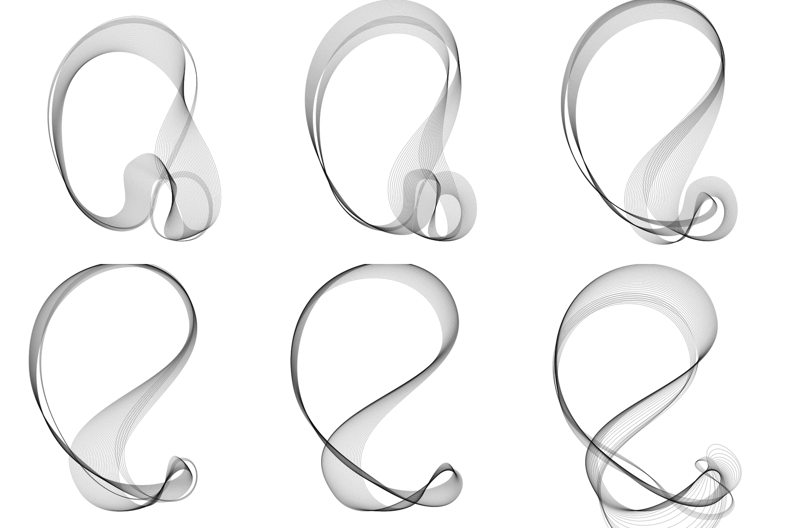
Swoopy lines flowing across the image, but with occasional jumps

I’ve used a single Hilbert sorter for all of the frames to remove some jumping, but the Hobby curves still hop around. Also the animation doesn’t loop smoothly, so there’s a giant jump from frame 100 back to frame 1.

Natural cubics

Hobby curves look nice, but have this unfortunate discontinuity where a small change in a point can lead to a radical change in the curve. There’s another way to compute curves through points automatically, called natural cubic curves. These curves don’t jump around the way Hobby curves can.

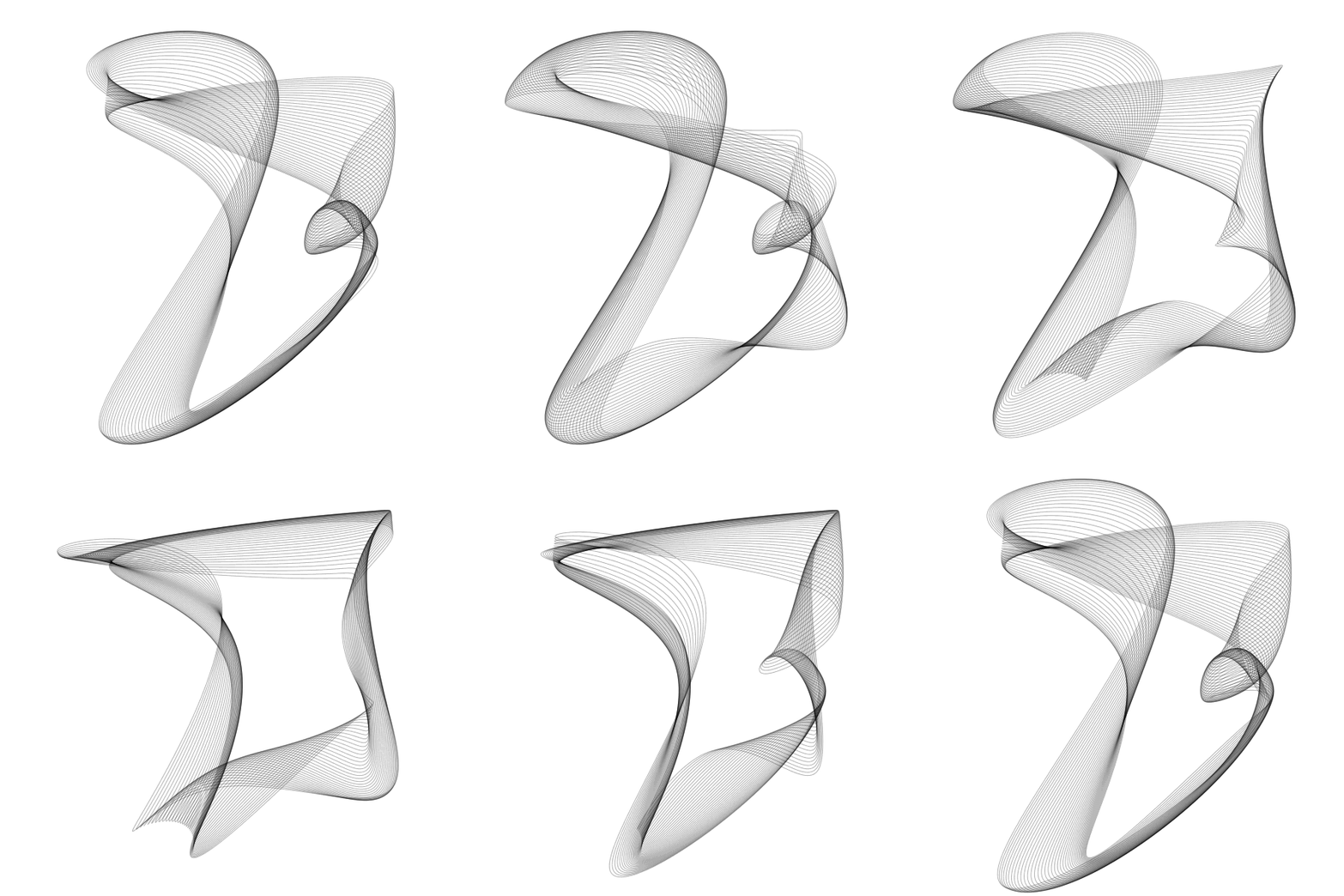
Jake Low’s page about Hobby curves has interactive examples of natural cubic curves which you should try. Natural cubics don’t look as nice to our eyes as Hobby curves. Below is a comparison. Each row has the same points, with Hobby curves on the left and natural cubic curves on the right:

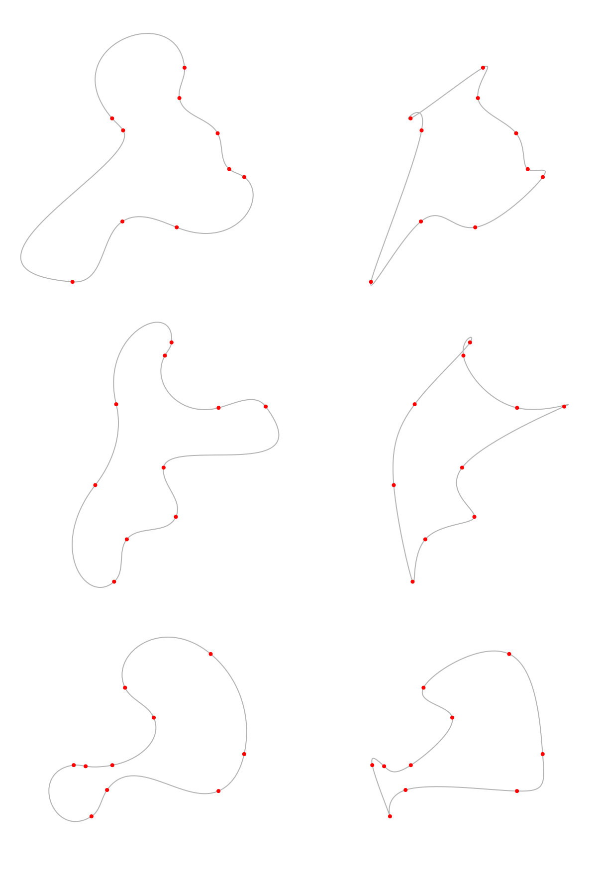
On the right are nice blobby shapes, on the left are the same points but connected with sometimes pointy awkward curves

The “natural” cubics actually have a quite unnatural appearance. But in an animation, those quirks could be a good trade-off for smooth transitions. Here’s an animation with the same points as our first one, but with natural cubic curves:

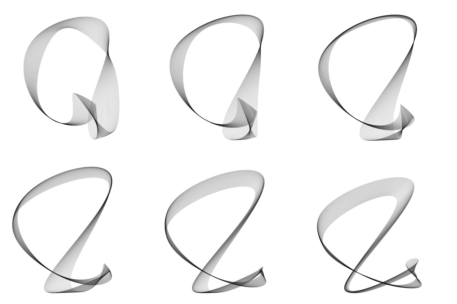
A flowing animation with pointier curves, only one jump at the end

Now the motion is smooth except for the jump from frame 100 back to frame 1. Let’s do something about that.

Circular Simplex

So far, we’ve been choosing points by sampling the simplex noise in small steps along a horizontal line: use a fixed u value, then take tiny steps along the v axis. That gave us our x coordinates, and a similar line with a different u value gave us the y coordinates. The ending point will be completely unrelated to the starting point. To make a seamlessly looping animation, we need our x,y values to cycle seamlessly, returning to where they started.

We can make our x,y coordinates loop by choosing u,v values in a circle. Because the u,v values return to their starting point in the continuous simplex noise, the x,y coordinates will return as well. We use two circles: one for the x coordinates and another for the y. The circles are far from each other to keep x and y independent of each other. The size of the circle is determined by the distance we want for each step and how many steps we want in the loop.

Here are three point paths created two ways, with linear sampling on the right and circular sampling on the left. Because simplex provides values between -1 and 1, the points wander within a square:

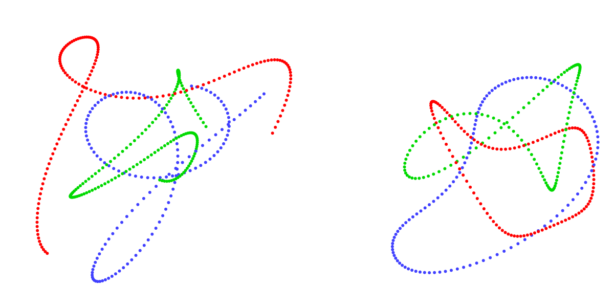
On the right, three trails of points that don't form a closed loop. On the left, three closed loops but still with interesting random shapes

It can get a bit confusing at this point: these traces are not the curves we are drawing. They are the paths of the control points for successive curves. We draw curves through corresponding sets of points to get our animation. The first curve connects the first red/green/blue points, the second curve connects the second set, and so on.

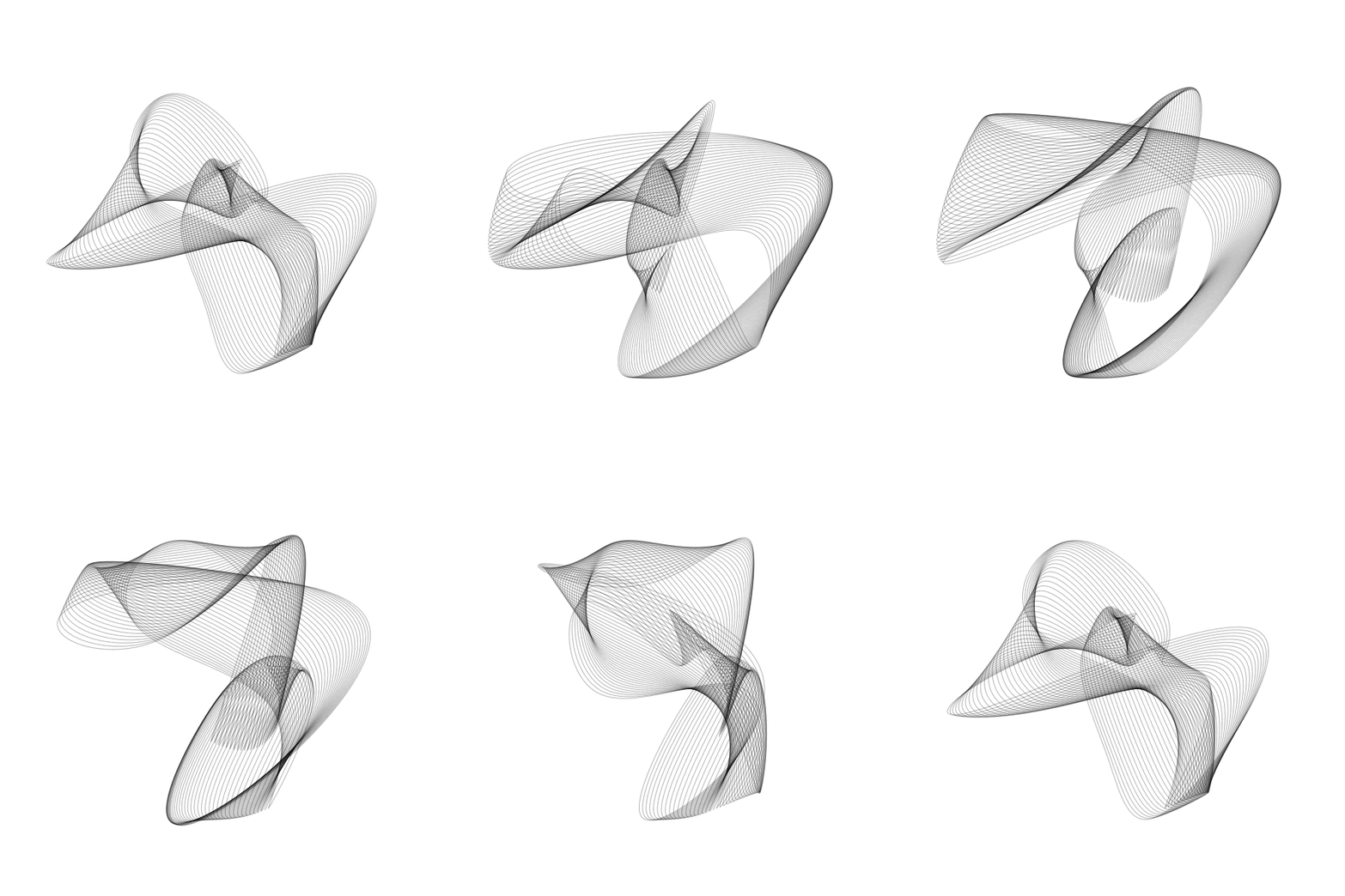
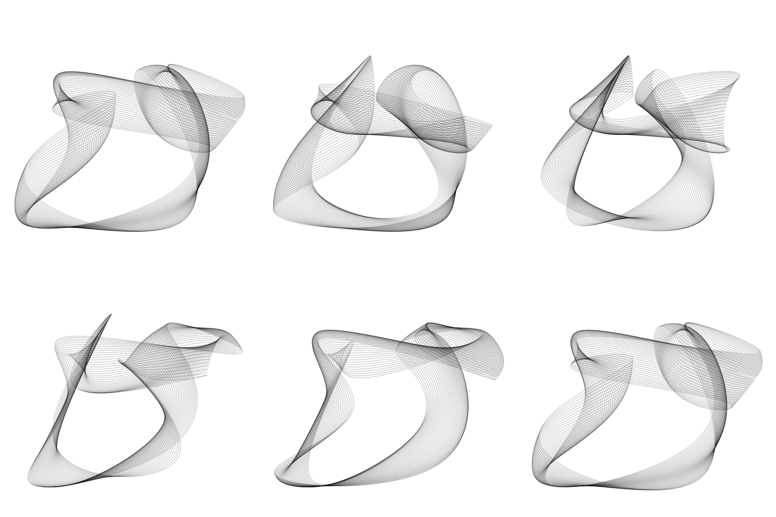
Using circular sampling of the simplex noise, we can make animations that loop perfectly:

Colophon

If you are interested, the code is available on GitHub at nedbat/fluidity.

Natural cubics, circular Simplex